A Time-Symmetric Model of Expansion and Renewal

1. Introduction

We develop a quantum–geometric cosmology in which two time–reversed branches form a globally zero–energy configuration. On the observed branch, the onset of classical history is identified with an emergence/partition event at \(t=0\). The emergence event marks the point at which a branch-normalized sector decomposition becomes physically meaningful. Although the logistic composition law introduced below admits analytic continuation as a function of \(t\), we take its physical domain on any single classical branch to be a finite interval

beginning at emergence and closing at a non-arbitrary endpoint \(t=L\) fixed by the midpoint symmetry about dark–sector equality (Sec. Framework Overview). Times outside this interval are treated as bookkeeping continuation (e.g. into a conjugate branch) rather than as an extension of a single classical history.

In the remainder we adopt the mirror-closed convention,

as the canonical branch-epoch length. An alternative operational definition based on dark-energy exhaustion, \(L_{\varepsilon}\), is introduced in Sec. Finite Epoch Exhaustion; for \(\varepsilon\ll 1\) this yields a longer epoch and serves as a phenomenological extension rather than a replacement of the mirror-closed construction.

At emergence, an asymmetric geometric seed,

fixes boundary data for the initial partition of the cosmic energy budget within a cube–circle construct.

Rescaled seed (two-quadrant deficit).

Because \(\alpha\) is the normalized circle–square deficit at the quadrant level, it reappears in rescaled form whenever the construction aggregates multiple identical quadrant gaps. In particular,

so occurrences of \(2-\pi/2\) should be read as a two-quadrant (half-scale) appearance of the same intrinsic seed, not as an additional independent input.

Geometric emergence fractions.

The cube–circle construction supplies the emergence partition

which sums to unity exactly. We interpret \(\Omega_{\rm de}\) as vacuum-like coherence and \(\Omega_{\rm dm}\) as localized gravitating structure emerging through decoherence. The baryonic weight \(\Omega_b\) is taken as fixed by the geometric partition once the branch becomes classical.

A central point of the construction is the separation between (i) a finite conversion capacity supplied by geometry (the fixed dark-sector budget \(1-\Omega_b\)) and (ii) a time profile for redistribution supplied by a bounded law of motion. The seed asymmetry \(\alpha\) supplies boundary data at \(t=0\); it does not, by itself, prescribe the steepness or duration of conversion. The temporal unfolding is encoded instead by a normalized logistic composition variable whose midpoint is fixed by definition to coincide with dark–sector equality.

Dark–sector logistic and equality midpoint.

Let

denote the total dark–sector weight. In the minimal closed–epoch realization adopted here, \(S\) is taken constant over the decoherence/conversion epoch. Define the dark–matter share of the dark sector by

We postulate a logistic evolution on the physical branch-epoch \(t\in[0,L]\),

where \(\kappa\) sets the steepness and \(\gamma\) is the midpoint time. By construction,

so the inflection point of the S–curve is the epoch of dark–sector equality and the moment of maximal conversion rate.

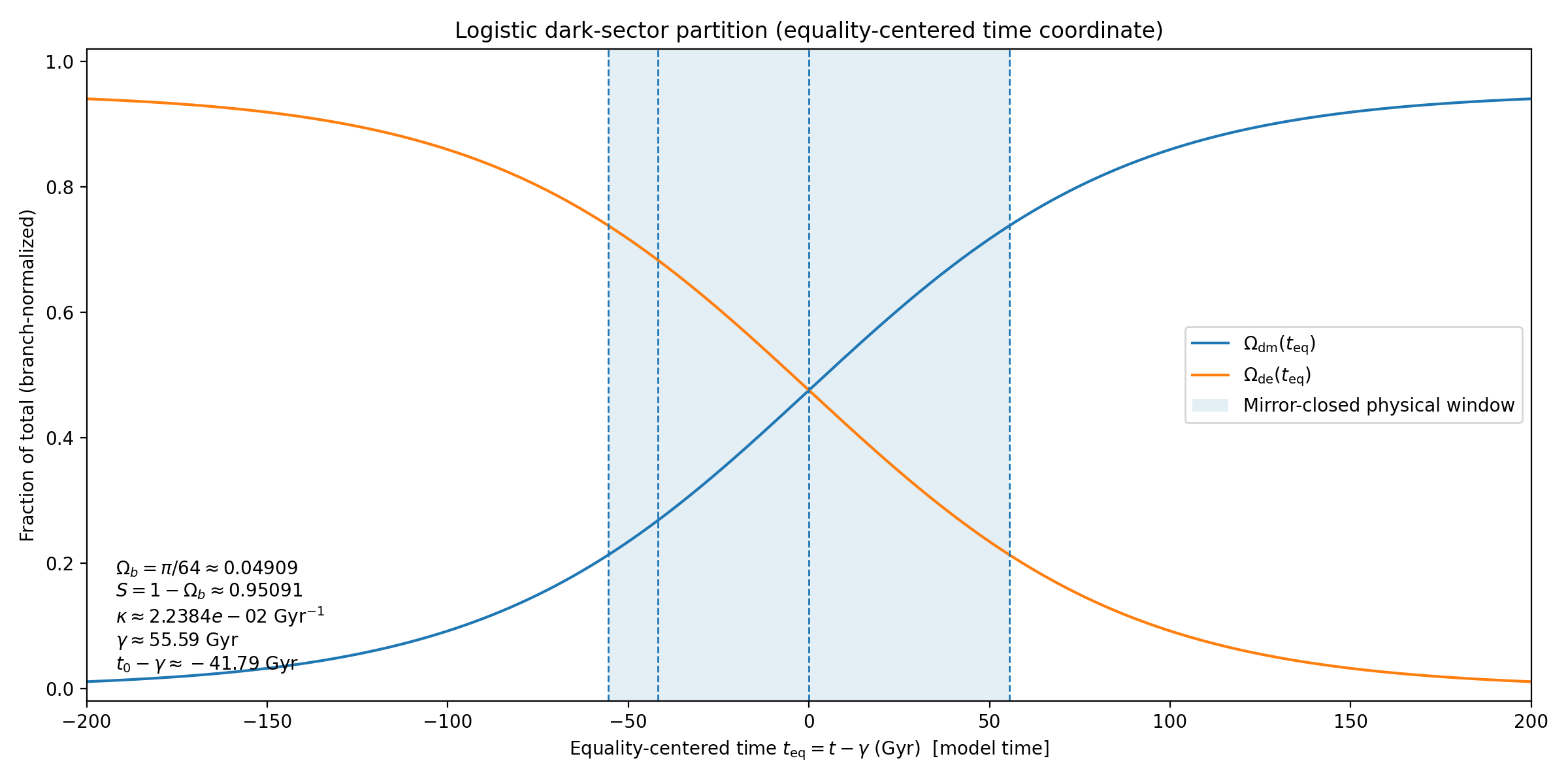
Equality-centered plotting coordinate.

For visual symmetry it is convenient to introduce an equality-centered time coordinate

so that the logistic composition law can be written as

with dark-sector equality at \(t_{\rm eq}=0\). The mirror-closed branch-epoch \(t\in[0,L_{\rm m}]\) with \(L_{\rm m}\equiv 2\gamma\) corresponds to the symmetric interval

where \(t_{\rm eq}=-\gamma\) is the emergence boundary (\(t=0\)) and \(t_{\rm eq}=+\gamma\) is its mirror endpoint (\(t=2\gamma\)). We retain \(t\) (with \(t=0\) at emergence) as the default time coordinate in the main text, and use \(t_{\rm eq}\) primarily for symmetric plots and schematics.

Mirror-closed epoch (finite completion without a terminus).

A logistic approaches \(f\to 1\) only asymptotically, so we do not define completion by an exhaustion threshold. Instead we use the exact complement symmetry of the logistic about \(\gamma\):

We define the end of a branch-epoch as the mirror of the emergence time \(t=0\) about the equality midpoint,

so that

Thus a single decoherence/conversion epoch is the interval \(t\in[0,L]\), closing at a non-arbitrary mirror state fixed by the equality midpoint. Accordingly, in figures and parameter anchoring we display and interpret the logistic history only on \(t\in[0,L]\); values outside this window represent formal continuation (or the conjugate branch under the complement rule) rather than an extension of the same classical branch.

Two-branch cyclicity.

Cyclicity is realized by a two-branch complement relation rather than by forcing \(f\) to reach \(0\) or \(1\) in finite time. Let \(f_+(t)\) denote the logistic share on the observed branch. Define the conjugate branch by

Equivalently, one may encode the alternation on a single bookkeeping time parameter as

The full cyclic period (return to the same partition) is therefore

Present–day anchoring.

Given an initial partition \((\Omega_{\rm dm}(0),\Omega_{\rm de}(0))\) at \(t=0\) and a present anchor \((\Omega_{\rm dm}(t_0),\Omega_{\rm de}(t_0))\) at \(t=t_0\), the logistic parameters are determined by the corresponding shares \(f(0)=\Omega_{\rm dm}(0)/S\) and \(f(t_0)=\Omega_{\rm dm}(t_0)/S\):

For the numerical values used in this work,

so that

This fixes where the present epoch lies on the S–curve and fixes the epoch closure time \(L\) by symmetry about the equality midpoint.

Baryonic emergence and bidirectional Viète structure.

The baryonic weight is fixed at emergence by \(\Omega_b=\pi/64\). To encode a percent-level residual associated with bidirectional circle–square closure, we introduce the dimensionless Viète-inspired factor

which parametrizes a small geometric imbalance between dual curvature projections. In this way, \(\alpha\) fixes the existence of an intrinsic seed asymmetry at \(t=0\), while \(\beta_{\mathrm V}\) provides a structural measure of finite residuals available to bias baryonic selection in the emergence partition. The logistic conversion profile remains a separate dynamical postulate governing dark-sector redistribution after emergence.

Notation and normalizations.

We set \(c=1\). The present cosmic age is \(t_0=13.8~\mathrm{Gyr}\). All sector quantities \(\Omega_i\) are branch-normalized weights satisfying Eq. (\ref{eq:branch_norm}) for \(t\ge 0\). We use \(\Omega_i\) as dimensionless sector weights; in the late-time FRW embedding (Sec. Einstein Conservation onward) they coincide with the usual critical-density fractions, but are not assumed to obey independent \(\Lambda\)CDM conservation laws because the dark components exchange energy.

Equality-centered time coordinate.

For visual symmetry it is convenient to introduce an equality-centered time

so that the logistic becomes \(f(\tau)=\bigl(1+e^{-\kappa\tau}\bigr)^{-1}\) with equality at \(\tau=0\). The mirror-closed epoch \(t\in[0,2\gamma]\) corresponds to \(\tau\in[-\gamma,+\gamma]\).

Imperfect symmetry and the origin of decoherence.

A guiding premise of this work is that perfectly realized symmetry is a singular idealization: in any finite–resolution physical system, exact symmetry does not generically select a preferred direction in state space, and therefore does not by itself supply an intrinsic notion of temporal ordering. Dynamical behavior requires not an externally imposed symmetry breaking, but the unavoidable presence of an intrinsic asymmetry arising from finite geometric realization.

In the present model this irreducible deviation is encoded at the emergence event \(t=0\) through the asymmetric seed \(\alpha\), which fixes boundary conditions for the initial partition of the cosmic energy budget. Crucially, \(\alpha\) does not by itself prescribe the conversion duration; it supplies nonzero boundary data from which subsequent redistribution within the dark sector proceeds.

The distinction between the existence of an asymmetry (boundary data) and its propagation (a law of motion) is essential. Accordingly, after emergence the conversion dynamics are encoded by the bounded logistic evolution of the dark–sector share \(f(t)\), whose midpoint is defined at dark–sector equality and whose epoch completion is defined by mirror closure at \(t=L=2\gamma\). Cyclicity is implemented by the two-branch complement rule. This separation of roles ensures that late–time behavior is insensitive to microscopic details of emergence while remaining predictive once the boundary data and present-day anchor are specified.

2. Underlying Number Theory: From Discrete Arithmetic to Spectral Quantum Geometry

2.1. Introduction

A quantum-geometric description of spacetime can be constructed from a small set of number-theoretic primitives. The constants \(1\), \(\sqrt{2}\), and \(\pi\) represent successive layers of algebraic and geometric structure that, when interpreted through spectral geometry and discrete-to-continuum physics, offer an arithmetic foundation for quantum spacetime. This section develops that viewpoint and frames these constants as generators of increasingly rich geometric and physical behavior.

2.2. The Unit \(1\): Discreteness, Quantization, and Arithmetic Foundations

The number \(1\) is the generator of discrete arithmetic. As the minimal unit of measure, it defines the foundation of quantization: all integer-valued observables—energy levels, occupation numbers, and topological charges—emerge from repeated addition of \(1\). The arithmetic structure of \(\mathbb{Z}\) thus functions as the primordial “quantum lattice.”

When extended to higher-dimensional integer lattices \(\mathbb{Z}^n\), the unit provides a combinatorial scaffold on which more complex geometric structures can be built. In spectral geometry, operators defined on such discrete lattices yield spectra that approximate continuous operators in appropriate limits. Thus, \(1\) encodes the discreteness from which continuum quantum geometry can be reconstructed.

2.3. The Irrational \(\sqrt{2}\): Algebraic Extension and the Birth of Geometry

The first nontrivial number-theoretic extension arises with \(\sqrt{2}\), the diagonal of the unit square. Its irrationality signals the emergence of geometric structure beyond the rationals. In arithmetic terms, the field extension \(\mathbb{Q} \to \mathbb{Q}(\sqrt{2})\) introduces irrationality as a structural necessity for Euclidean geometry.

Physically, \(\sqrt{2}\) represents the transition from discrete combinatorics to metric geometry. The Euclidean norm in \(\mathbb{R}^2\), normalization of two-state quantum systems, and the Hilbert-space inner product all implicitly rely on \(\sqrt{2}\). Quantum interference naturally introduces normalization factors of \(1/\sqrt{2}\), making \(\sqrt{2}\) the first irrational encoding orthogonality, metric relations, and vector structure in quantum Hilbert space.

In spectral terms, the Laplacian on a square lattice requires diagonal contributions whose geometric interpretation derives from the Pythagorean relation defining \(\sqrt{2}\). This connects algebraic irrationality to the eigenvalue structure of geometric operators, linking number theory to the spectral fingerprints of emergent space.

2.4. The Transcendental \(\pi\): Curvature, Rotation, and Phase Geometry

The constant \(\pi\) governs curvature and rotational symmetry. Unlike the algebraic number \(\sqrt{2}\), \(\pi\) is transcendental, signaling a conceptual leap from linear metric geometry to curved, rotational, and harmonic structures.

Angular momentum quantization, Fourier analysis, and the phase structure of quantum mechanics all rely on \(\pi\). The unitary evolution operator, expressed through complex exponentials, depends fundamentally on the periodicity of \(2\pi\), generating the \(U(1)\) phase symmetry underlying quantum wave behavior.

In spectral geometry, curvature and topology manifest through the spectra of differential operators. Heat kernels, spectral actions, and zeta functions all feature \(\pi\) in essential ways, linking transcendental number theory to physical predictions about spacetime geometry. Thus, \(\pi\) represents the arithmetic imprint of curvature, periodicity, and continuous rotational symmetry.

2.5. Spectral Geometry of Quantum Spacetime: An Arithmetic Perspective

The interplay among \(1\), \(\sqrt{2}\), and \(\pi\) provides a natural number-theoretic narrative for spectral geometry. In noncommutative and quantum-geometric models, spacetime is described through operator algebras in which geometric information is encoded spectrally rather than coordinately.

• Discrete spectra (arising from the integer structure of \(1\)) correspond to quantized observables.
• Quadratic forms and their irrational extensions (embodied by \(\sqrt{2}\)) determine the metric encoded by the Dirac or Laplace operator.
• Curvature and phase structure (governed by \(\pi\)) appear in spectral actions, heat-kernel coefficients, and oscillatory quantum amplitudes.

This progression mirrors the hierarchy of number theory itself: the rational, the algebraic, and the transcendental. Spacetime geometry emerges as the spectral synthesis of these arithmetic layers.

2.6. Discrete-to-Continuum Quantum Physics

Quantum geometry often begins with a discrete substrate—graphs, causal sets, integer lattices, or operator algebras—and recovers continuum physics in a spectral limit. The constants \(1\), \(\sqrt{2}\), and \(\pi\) encode the essential transitions:

• \(1\) \(\to\) the discrete quantum: the arithmetic lattice of states.
• \(1\) to \(\sqrt{2}\) \(\to\) the metric quantum: emergence of orthogonality, norm, and Euclidean geometry.
• \(\sqrt{2}\) to \(\pi\) \(\to\) the geometric quantum: emergence of curvature, rotation, and wave dynamics.

This arithmetic ladder reflects the physical pathway from quantum discreteness to smooth spacetime. Spectral geometry bridges these regimes: discrete Laplacians converge to continuous ones, eigenvalues approximate curvature, and algebraic structures converge toward geometric manifolds.

Thus, the number-theoretic constants serve as seeds for the full geometric machinery of quantum physics, shaping both the combinatorial microstructure and its continuum geometric limits.

2.7. Summary

The constants \(1\), \(\sqrt{2}\), and \(\pi\) form a natural arithmetic hierarchy mirroring the geometric structures required for quantum spacetime:

• \(1\) encodes discreteness and quantization.
• \(\sqrt{2}\) encodes orthogonality and metric relations.
• \(\pi\) encodes rotation, curvature, and phase.

Spectral geometry provides the bridge connecting these number-theoretic primitives to physical spacetime. In this view, quantum geometry emerges organically from arithmetic structure, with spectral operators translating numeric primitives into geometric form.

3. Framework Overview

We now formalize the geometric structure of the model using a cube–circle framework that encodes the balance between localization and coherence. The organizational principle is a strict separation between boundary data fixed at the emergence/partition event \(t=0\) and a bounded law of motion governing subsequent redistribution within the dark sector.

Cube–circle partition and sector identification.

The construction begins with a unit cube enclosing two opposed conic volumes defined by quarter–circular arcs. The resulting volumetric ratios,

define three branch-normalized sector weights at emergence, interpreted as baryonic matter (\(\Omega_b\)), dark matter (\(\Omega_{\rm dm}\)), and dark energy (\(\Omega_{\rm de}\)). These ratios are used throughout as a compact geometric encoding of complementary structure rather than as a literal spatial tessellation. In particular, the contrast between the circle (curvature/phase, \(\pi\)) and the square/cube (orthogonality/metric structure, \(\sqrt{2}\)) is used as a geometric analogue of the opposition between delocalized coherence and localized, particle-like curvature modes.

Emergence at \(t=0\) and the asymmetric seed.

The Big Bang is identified here with the emergence/partition event at \(t=0\), where the branch-normalized sector weights in the equation above become classically meaningful. The existence of a decoherence channel is traced to an intrinsic geometric mismatch between ideal rotational closure and finite orthogonal constructions, quantified by the circle–square deficit

This quantity is structural: it supplies the irreducible asymmetry required for a directed classical history to emerge, but it does not by itself prescribe the temporal profile of the subsequent conversion.

Dark–sector redistribution as a bounded logistic.

After emergence, the model focuses on redistribution within the dark sector while keeping the baryonic sector fixed by geometry. Define the dark sector total and the dark-matter share

so that \(\Omega_{\rm dm}(t)=S\,f(t)\) and \(\Omega_{\rm de}(t)=S[1-f(t)]\). In the minimal closed-epoch realization, \(S\) is taken constant over a decoherence/conversion epoch. The temporal unfolding is encoded by the logistic law

where \(\kappa\) sets the steepness and \(\gamma\) is the midpoint time. The midpoint is fixed by dark–sector equality:

Thus the inflection point of the S–curve is identified with the physically distinguished epoch at which the dark sector is exactly balanced and the conversion rate is maximal.

The conversion epoch as a finite interval on the S–curve.

Although a logistic approaches \(f\to 0\) or \(f\to 1\) only asymptotically, the framework admits a non-arbitrary finite epoch definition using the exact complement symmetry about the midpoint. We define the endpoint of a single branch-epoch as the mirror of \(t=0\) about \(t=\gamma\):

This choice implies \(f(L)=1-f(0)\) and therefore exchanges the emergence weights of the two dark components across the epoch: \(\Omega_{\rm dm}(L)=\Omega_{\rm de}(0)\) and \(\Omega_{\rm de}(L)=\Omega_{\rm dm}(0)\). In this model the Big Bang epoch refers to the decoherence/conversion interval \(t\in[0,L]=[0,2\gamma]\).

3.1. Radiation Era and Branch Normalization

The emergence/partition event at \(t=0\) is treated as the onset of a classical branch description in which sector weights can be assigned. Times \(t<0\) are interpreted as a pre-classical regime in which the order parameter exists but the sector decomposition is not yet operational. In this sense, the earliest radiation-dominated phase of standard cosmology is not modelled here as a time-dependent sequence of \(\Omega_i(t)\); instead, radiation is understood as a pre-partition (or rapidly transient post-partition) component that dilutes prior to the branch-normalized accounting adopted in the remainder of the work.

Accordingly, throughout this paper we use branch normalization

and treat the cube–circle ratios as boundary data at emergence, rather than as the \(a\to 0\) limit of FRW density fractions.

3.2. Geometric Instability, Decoherence, and the Seeded Boundary Condition

The circle–square deficit \(\alpha=1-\pi/4\) encodes a mismatch between ideal rotational coherence and finite orthogonal realizability. In the hypothetical limit \(\alpha\to 0\) (exact geometric closure), a perfectly symmetric coherent state would not generically select a preferred direction in state space. A nonzero \(\alpha\) renders perfect coherence only metastable, permitting a directed classical history to emerge once the sector partition becomes meaningful at \(t=0\).

In this formulation, the seed \(\alpha\) fixes only boundary data (the existence of an intrinsic asymmetry at emergence); it is not inserted as an explicit forcing term in the evolution law. The propagation of decoherence is encoded instead by the bounded logistic evolution of the dark share \(f(t)\). The midpoint of the S–curve is fixed by construction to coincide with dark-sector equality, while epoch completion is defined by mirror closure at \(t=L=2\gamma\). This separation of roles isolates (i) the geometric origin of asymmetry from (ii) the coarse-grained time profile by which it unfolds.

3.3. Baryonic Emergence from Bidirectional Viète Structure

In the cube–circle construction, the baryonic sector weight is fixed at emergence by \(\Omega_b=\pi/64\). To encode the presence of finite residuals in bidirectional circle–square closure, we introduce a Viète-inspired structural factor

and the associated percent-level residual

This \(\varepsilon_{\mathrm V}\) is interpreted as a geometric measure of finite-depth mismatch between dual curvature projections. In the present paper it serves as a compact structural parameter available to bias baryonic selection (or baryogenesis) within the emergence partition, while the subsequent dark-sector redistribution is governed independently by the logistic history \(f(t)\).

4. Dynamic Evolution Law

The cosmological evolution on a given branch is modelled as a bounded redistribution process within the dark sector: vacuum-like coherence (\(\Omega_{\rm de}\)) progressively converts into localized gravitating structure (\(\Omega_{\rm dm}\)), while \(\Omega_b\) remains fixed by the geometric emergence partition. The conversion coordinate is the dark-sector share \(f(t)=\Omega_{\rm dm}(t)/S\), whose midpoint is by definition the epoch of dark-sector equality.

4.1. Logistic Law with Equality Midpoint

With \(S=\Omega_{\rm dm}(t)+\Omega_{\rm de}(t)\) constant over an epoch and \(f(t)\equiv \Omega_{\rm dm}(t)/S\), we impose

so that

The logistic has an exact complement symmetry about \(\gamma\),

which will be used to define finite epochs and cyclic completion without requiring asymptotic exhaustion.

4.2. Conversion Rate and Dark–Sector Flux

Differentiating the logistic yields

so that (with \(S\) constant)

and hence

Windowed dynamics and epoch closure.

Because the exchange kernel is \(f(1-f)\), the conversion rate is symmetric about the equality midpoint and returns to the same value at mirror times:

This makes \(t\in[0,2\gamma]\) a natural closed conversion window: the epoch begins at emergence and closes at its mirror state without invoking asymptotic tails of the logistic outside the physical branch interval. The conversion rate is uniquely maximized at equality \(f=\tfrac12\), where

Anchoring by boundary data and one present-day point.

The steepness \(\kappa\) and midpoint \(\gamma\) are fixed by requiring that the logistic passes through (i) the emergence share \(f(0)\) implied by the cube–circle partition and (ii) a present-day anchor \(f(t_0)\) at \(t=t_0\):

This uniquely determines where the present epoch lies on the S–curve.

4.3. Mirror-Closed Epoch and Big Bang Duration on the S–Curve

A logistic does not reach \(f=0\) or \(f=1\) in finite time, but it does admit a natural finite epoch definition via symmetry. We define the end of a single branch-epoch as the mirror of \(t=0\) about the midpoint \(t=\gamma\):

Then

In this framework, the Big Bang epoch is the finite conversion interval \(t\in[0,L]\), i.e. the portion of the S–curve between emergence and its mirror state about dark-sector equality.

4.4. Time–Reversal Pairing and Two–Branch Completion

Let \(f_+(t)\) denote the logistic composition history on the observed branch for \(t\in[0,L_{\rm m}]\), with \(L_{\rm m}\equiv 2\gamma\). Define the conjugate (time–reversed) branch to traverse the same S–curve in the opposite direction:

Using the logistic complement symmetry about \(\gamma=L_{\rm m}/2\), this is equivalently

Differentiating gives the conversion-direction reversal in each branch's forward time:

where the second equality uses \(\dot f(L_{\rm m}-t)=\dot f(t)\). Thus the two branches share the same conversion magnitude but carry opposite conversion direction.

4.5. Quantum–Geometric Interpretation

At \(t=0\) the sector partition becomes classical and is fixed by the cube–circle boundary data, seeded by the intrinsic asymmetry \(\alpha=1-\pi/4\). Subsequent history on a given branch is governed by the bounded logistic conversion \(f(t)\), interpreted as progressive decoherence of vacuum-like coherence into localized gravitating structure within the fixed dark-sector budget \(S=1-\Omega_b\). The equality midpoint \(t=\gamma\) is distinguished by maximal conversion rate and exact dark-sector balance, and the conversion epoch is identified with the finite S-curve interval \(t\in[0,2\gamma]\) terminating at the mirror state of emergence. In a two-branch completion, the conjugate branch carries the complementary conversion direction, enabling cyclic closure through the relation \(f_-(t)=1-f_+(t)\) while preserving a globally time-symmetric, zero-energy picture.

5. Cyclic Symmetry

The cyclic (time–symmetric) completion of the baseline model can be presented in two equivalent endpoint conventions: (i) a mirror-closed branch-epoch with endpoint \(L=2\gamma\) fixed by complement symmetry about the equality midpoint, and (ii) an operational endpoint \(L_{\varepsilon}\) defined by a dark–energy exhaustion threshold \(f(L_{\varepsilon})=1-\varepsilon\) (Sec. Finite Epoch Exhaustion). The mirror-closed realization used in the geometric construction is the special case \(\varepsilon=f(0)\), for which \(L_{\varepsilon}=2\gamma=L\) and the dark components exchange their emergence weights across the epoch.

Branch pairing and the equality midpoint.

Let \(M_+\) denote the observed expansion branch, emerging at \(t=0\) and evolving monotonically according to the logistic history. The equality midpoint is the (unique) time at which the dark components coincide:

The end of the finite epoch on \(M_+\) is defined by the exhaustion threshold \(\Omega_{\rm de}(L)=\varepsilon S\) (equivalently \(f(L)=1-\varepsilon\)).

The conjugate partner branch \(M_-\) is introduced by reflecting the coordinate time about the equality midpoint,

together with the complement symmetry of the logistic coordinate,

Equation \(f(2\gamma-t)=1-f(t)\) exchanges the roles of dark matter and dark energy at conjugate times. Differentiating gives the kernel symmetry

so the magnitude of the conversion rate is symmetric about equality. The direction of conversion nevertheless reverses when one differentiates with respect to each branch’s own forward time parameter. In this way, the paired branches carry opposite conversion directions while retaining equal conversion magnitudes under the global pairing.

Finite epoch and cycle completion.

On a single branch the logistic dynamics require no sign flip of \(\kappa\). Instead, the conversion epoch is taken to be finite by definition: it terminates once dark energy falls below the exhaustion threshold, \(\Omega_{\rm de}(L_{\varepsilon})=\varepsilon S\) (equivalently \(f(L_{\varepsilon})=1-\varepsilon\)). The corresponding duration \(L\) is finite. In this sense, “cyclic” refers to the existence of a bounded conversion interval within each branch, together with the time–reversal pairing needed for the global zero–energy completion.

Equality is built in.

Because the logistic coordinate is the dark–sector share \(f(t)\), the model identifies the logistic inflection point with the equality epoch: both occur at \(t=\gamma\). Thus there is no separation between “maximum conversion rate” and “dark equality” within the present parameterization; equality is encoded directly as the midpoint condition.

5.1. Entanglement Interpretation of the Renewal Phase

Within the time–symmetric completion, one may interpret the renewal branch as the quantum–conjugate mirror of the observed cosmological domain. A convenient schematic representation is a balanced superposition of two time–reversed sectors,

where \(|\Psi_{+}\rangle\) corresponds to \(M_+\) and \(|\Psi_{-}\rangle\) to its conjugate partner \(M_-\). In a globally zero–energy construction, one envisions that suitable expectation values can cancel between the conjugate sectors so that the composite two–branch state is energy neutral, even though each branch supports a locally time–directed semiclassical history.

In this interpretive picture the mirror sector need not be viewed as a separate classical universe; it can instead be treated as a conjugate component of a single quantum–geometric state. Residual entanglement between sectors then acts effectively as curvature within each branch. As decoherence proceeds away from the emergence boundary at \(t=0\), cross–branch interference is suppressed and the effective dynamics within each branch become increasingly local and semiclassical. Near the equality midpoint \(t=\gamma\), the global pairing symmetry extremizes cross–branch correlations; in speculative renewal scenarios, this locus may be a natural site to discuss re–coherence mechanisms that could seed a subsequent epoch.

This interpretation is not required for the baseline logistic dynamics, but it provides a quantum–informational narrative linking the zero–energy completion, the time–reversed pairing, and the emergence of branch–local gravitational phenomenology from residual cross–correlations. The factor \(1/\sqrt{2}\) simply encodes the balanced weighting of a symmetric two–branch superposition in this schematic representation.

6. Physical Interpretation

The framework admits a compact physical reading in which (i) global energy neutrality is implemented through a two–branch completion, (ii) the dark sector is modeled as a bounded decoherence/re–coherence channel, and (iii) the salient times are fixed by definition (equality midpoint) and by threshold (exhaustion endpoint), rather than by an arbitrarily imposed time window.

• Zero–Energy Completion. The construction assumes that the universe admits a globally balanced (net–zero) energy accounting when matter–energy is combined with gravitational contributions. This motivates a time–reversed pairing in which two conjugate branches may contribute equal and opposite energetic components when considered as a composite configuration. Each branch remains locally time–directed, while the two–branch completion is formally time symmetric.
• Residual Cross–Branch Correlations. In the time–symmetric extension, gravity may be interpreted as a weak residual correlation between conjugate branches \(M_+\) and \(M_-\). In the schematic superposition, cross–branch entanglement can be viewed as producing an effective curvature response within each branch without modifying the baseline logistic conversion law.
• Dark Components and the Equality Midpoint. Dark matter and dark energy are treated as complementary manifestations of vacuum (de)coherence: dark matter as localized, gravitating curvature modes and dark energy as a delocalized coherence reservoir. Their relative magnitudes are tracked by the dark–sector share \(f(t)=\Omega_{\rm dm}/(\Omega_{\rm dm}+\Omega_{\rm de})\) (equivalently \(f=\Omega_{\rm dm}/S\) when \(S\) is constant within an epoch). A defining feature of the parameterization is that the logistic midpoint is fixed by construction to coincide with dark–sector equality: \[ f(\gamma)=\tfrac12 \quad\Longleftrightarrow\quad \Omega_{\rm dm}(\gamma)=\Omega_{\rm de}(\gamma)=\frac{S}{2}. \] Thus the theory singles out a preferred crossing time as an intrinsic geometric feature of the coordinate choice, rather than as an incidental output of a fit.
• Exhaustion Endpoint and Finite Epoch Structure. On a single branch the epoch is finite by definition: it terminates when dark energy falls below a small exhaustion fraction \(\varepsilon\ll 1\), \(\Omega_{\rm de}(L)=\varepsilon S\) (equivalently \(f(L)=1-\varepsilon\)). This defines an operational end time \(L\) and hence a cycle–completion criterion within the branch. Strong renewal (re–coherence and re–seeding) is an additional dynamical hypothesis, but the baseline model already provides the canonical markers: emergence at \(t=0\), equality at \(t=\gamma\), and completion at \(t=L\).
• Thermodynamic Arrow. Entropy increases monotonically along each individual branch, reflecting the irreversibility of decoherence in forward physical time. In a formally time–symmetric completion, the conjugate branch provides the time–reversed counterpart, so that the composite description admits a global bookkeeping symmetry under time reversal. Whether this symmetry corresponds to a realized physical re–coherence cycle or merely to a completion principle depends on physics beyond the baseline logistic evolution.

Together, these elements define a quantum–geometric cosmology in which the emergence event at \(t=0\) is seeded by the intrinsic asymmetry \(\alpha=1-\pi/4\), the subsequent dark–sector redistribution is governed by a bounded logistic whose midpoint is dark–sector equality, and finite epoch completion is defined by dark–energy exhaustion. Baryonic emergence is anchored independently by the bidirectional Viète recursion factor \(\beta=9\sqrt{2}/(4\pi)\), linking geometry, energy, and information within a single manifold.

7. Observational Outlook

The framework suggests observational handles that could, in principle, distinguish it from conventional \(\Lambda\)CDM phenomenology if residual coherence, cross–branch correlations, or renewal dynamics are realized in nature. Independent of any particular dataset fit, the model adds a qualitative structural statement not present in standard parameterizations: it places the present universe within a finite conversion window bounded by emergence at \(t=0\) and exhaustion at \(t=L\), with a physically defined midpoint \(t=\gamma\) set by dark–sector equality.

Possible phenomenological consequences include:

• Mass–to–Light Systematics. If decoherence is incomplete or spatially nonuniform, regions of partial vacuum coherence could persist. This may appear as correlated deviations in inferred mass–to–light ratios and/or environmental trends in dark–matter inferences relative to standard expectations.
• Gravitational–Wave Background Structure. If coherent restructuring of curvature is enhanced near the equality epoch \(t=\gamma\) or during a putative renewal phase, the resulting dynamics could source distinctive low–frequency gravitational–wave backgrounds. In this picture, such signals would trace large–scale geometric realignment rather than purely stochastic astrophysical superposition.
• Neutrino Phase Sensitivity. If residual inter–branch correlations persist in any effective description, they could manifest as small phase shifts or oscillation anomalies in high–energy neutrino populations, providing an indirect probe of coherence beyond the minimal particle–physics framework.
• Redshift Evolution of the Dark–Sector Ratio. Because the midpoint is fixed by equality and the endpoint by exhaustion, the model predicts a specific evolution of \(\Omega_{\rm dm}/\Omega_{\rm de}\) once the mapping between cosmic time \(t\) and the scale factor \(a(t)\) is specified. Constraints on the redshift dependence of effective dark–energy behavior therefore provide a direct test of the logistic conversion hypothesis.

Collectively, these avenues share a common premise: if late–time observables retain any memory of an underlying quantum–geometric origin, then precision measurements of gravitational–wave spectra, galactic dynamics, neutrino oscillation phases, and redshift–dependent dark–sector behavior may expose deviations from purely classical parameterizations.

8. Quantum–Correlative Interpretation

In the time–symmetric extension, one may view the late–time universe as comprising two semiclassical branches related by time reversal, with decoherence suppressing direct interference but not necessarily eliminating all cross–correlations. In this reading, phenomena attributed to dark matter and dark energy arise as effective semiclassical manifestations of residual correlations between two conjugate branches in a globally zero–energy completion. No additional exotic particles or ad hoc vacuum fields are assumed beyond the geometric vacuum response already encoded in the branch–normalized dark sector.

Within this interpretation, dark–sector phenomenology corresponds to the primary stage of cosmological decoherence: delocalized vacuum coherence is progressively converted into localized, gravitating curvature modes. In the dynamical model developed above, this conversion is tracked by the dark–sector share

whose logistic midpoint is fixed by equality and whose endpoint is fixed by exhaustion. The emergence event at \(t=0\) is then the moment at which the seeded asymmetry \(\alpha=1-\pi/4\) renders perfect coherence metastable and selects the initial partition of sectors.

Baryonic emergence and secondary localization.

Baryonic matter may be interpreted as a secondary localization channel within an already decohering dark sector, preferentially realized inside gravitational wells. In the geometric formulation, baryonic emergence is anchored not by the dark–sector logistic itself but by the bidirectional Viète recursion factor

which encodes a percent–level curvature asymmetry selecting a small branch–normalized baryonic fraction at emergence. On this view, the dark sector provides the large–scale gravitational scaffold, while baryons represent a further stage of localization that becomes dynamically relevant once structure formation amplifies curvature gradients.

Although the composite two–branch state is taken to be globally unitary in this extension, local observers have access only to a decohered sector and therefore experience effective probabilistic outcomes and a monotonic entropy increase. In a curved spacetime with a seeded asymmetry, limited access to global correlations can support the emergence of locally ordered structures—including self–organizing and biological complexity—without violating the second law, because the corresponding entropy budget is exported into inaccessible degrees of freedom that remain correlated at the level of the composite state.

Thus, apparent randomness and structure formation can be viewed as natural byproducts of a globally time–symmetric quantum state once observers are restricted to a single decohered branch.

8.1. Black Holes as Bidirectional Quantum Boundaries

In a globally pure, time–symmetric quantum description, decoherence separates the universe into two semiclassical branches related by time reversal. Observers confined to a given branch access only a reduced description of the total state, and this restriction manifests as apparent information loss and a monotonic thermodynamic arrow. Black holes provide an extreme setting in which this restriction is sharpened: horizons act as high–curvature boundaries that limit branch–local access to quantum information while remaining compatible with global unitarity in the two–branch completion.

From the conjugate (time–reversed) branch viewpoint, the same horizon can be interpreted as a boundary across which correlations are redistributed rather than destroyed. In this sense, degrees of freedom that appear inaccessible on one branch may correspond to degrees of freedom encoded differently in its conjugate partner, consistent with the premise that the composite state remains unitary even when each semiclassical branch admits an effectively irreversible thermodynamic description.

This bidirectional role motivates viewing black holes as entanglement nodes linking correlated semiclassical histories. Their curvature extremality and causal structure make them natural loci at which cross–branch correlations might be concentrated, while still forbidding superluminal signalling and preserving semiclassical causality within either branch individually.

Within the present interpretive extension, black holes therefore function as decoherence surfaces for observers restricted to a single semiclassical history, and simultaneously as candidate re–encoding (or re–coherence) boundaries in the conjugate sector. This preserves global time symmetry at the level of the composite state while offering a quantum–correlative narrative for gravitational phenomenology, including the persistence of dark–sector effects after direct interference has been suppressed by decoherence.

9. Viète’s Product as a Structural Geometric Archetype

Viète’s infinite product for \(\pi\) plays no direct dynamical role in the cosmological construction developed below. Its role is structural: the recursion provides a clean geometric archetype of how complementary (dual) operations can converge to a globally symmetric limit while any finite truncation retains a nonzero residual. This is the qualitative pattern we later reuse when motivating a globally neutral (zero–energy) universe completed by a conjugate, time–reversed partner branch.

Interpretive remarks—including possible connections to mirror dualities and time–reversed branches—are deferred to Appendix Mirror \(\pi\). In the main text we require only the circle–square residual

used as a dimensionless seed of geometric asymmetry, without invoking any dual–valued or otherwise nonstandard extensions of \(\pi\).

10. The Circle–Square Gap as a Finite Residual Asymmetry

Viète’s product exemplifies a useful geometric property: iterative curvature corrections can approach a symmetric limit while leaving a finite discrepancy at any finite stage. In the present framework, this “finite residual” motif is reused in two places: first as the circle–square gap \(\Delta\), and later as a smaller bidirectional remnant \(\varepsilon_{\mathrm V}\).

Consider a circle of radius \(r\) inscribed in a square of side \(2r\). Their areas are

so the scale–free fractional difference is

For later reference, the corresponding half-scale (two-quadrant) deficit is simply \(2-\pi/2=2\Delta=2\alpha\). Equivalently, the same residual appears in additive (unnormalized) form as \(A_\square-A_\circ = 4r^2\,\alpha\). For \(r=1\) one has \(4-\pi=4\alpha\), while the half-area version is \(2-\pi/2=2\alpha\).

Numerically, \(\Delta\simeq 0.2146\) provides a minimal measure of the mismatch between orthogonal (square) and rotational (circular) geometry. In the cosmological model, this finite residual is used only as boundary data at \(t=0\): it seeds the initial asymmetry from which the subsequent dark–sector evolution proceeds.

Rescaled forms of the seed.

Because \(\alpha\) is the normalized circle–square deficit at the quadrant level, it reappears in rescaled form whenever the construction aggregates multiple identical quadrant gaps. In particular,

so the same intrinsic asymmetry contributes twice in any two-quadrant (half-scale) geometric closure. Throughout we treat \(\alpha\) as the fundamental seed parameter; expressions such as \(2-\pi/2\) are not new inputs but simple rescalings of the same geometric residual.

10.1. Viète’s Product as a Recursive Dual Closure

Viète’s formula,

arises from repeated half–angle refinement of inscribed regular polygons. Each cosine may be viewed as a curvature–projection factor that reduces the discrepancy between polygonal and circular geometry. The essential point for us is not the numerical value of \(\pi\) but the structure of the recursion: the infinite limit achieves an invariant, while any finite truncation retains a residual discrepancy.

This limit–preserving structure motivates, at the level of geometric intuition, how a globally neutral (zero–energy) completion can remain compatible with finite, locally meaningful asymmetries.

10.2. Expressing the Gap Through Viète–Like Closure

Inverting the product and rescaling yields a nested–radical representation of \(\pi/4\),

so the gap may be written equivalently as

Each nested radical encodes one stage of progressive curvature reconciliation. The infinite limit removes the discrepancy entirely; the finite remainder at any intermediate depth is a geometric analogue of a finite, dynamically relevant asymmetry.

10.3. Finite Residuals and a Zero–Energy Bookkeeping

The pair \(\bigl(2/\pi,\;1-2/\pi\bigr)\) provides a complementary partition of unity and will be used only as a mnemonic for “complementary sectors” in the later time–symmetric completion. In a zero–energy bookkeeping one needs an antisymmetric (sign–reversing) combination between conjugate branches; a natural such combination is the centered deviation

One may then schematically assign opposite contributions to conjugate sectors,

emphasizing that the use of \(\pi\)–weights here is purely symbolic: it serves only to illustrate how exact global cancellation can coexist with finite residuals at the level of individual components.

10.4. A Bidirectional Circle–Square Construction

Viète’s recursion is a one–sided inward convergence. For cosmological intuition it is useful to consider a bidirectional analogue: inscribe a circle in a square and circumscribe a square about that circle. In linear scale these correspond to conjugate factors \(1/\sqrt{2}\) (contraction) and \(\sqrt{2}\) (expansion).

Treating these as reciprocal amplitudes of a single geometric transformation and adopting a volumetric normalization (hence the cube), define

and identify this dimensionless factor with the bidirectional Viète emergence parameter,

Its deviation from unity,

quantifies the first nontrivial residual imbalance between the dual curvature projections. In the cosmological model, \(\varepsilon_{\mathrm V}\) is used as a compact geometric seed for a small local offset within each semiclassical branch.

10.5. Successive Refinements and Rapid Suppression

The bidirectional construction can be refined by replacing the elementary \(\sqrt{2}\) step by deeper Viète–style curvature refinements (equivalently, higher–depth polygonal approximations). The key qualitative outcome is robust: as the refinement depth increases, the residual mismatch between complementary curvature projections is suppressed rapidly. Operationally, this provides a controlled way to generate a small but nonzero geometric remnant at finite depth, while retaining a well–defined symmetric limit in the infinite refinement.

10.6. Local Asymmetry in a Globally Symmetric Universe

In the time–symmetric completion, global symmetry is implemented at the level of the two–branch state,

with total energy and curvature taken to cancel across the conjugate pair. The geometric residual \(\varepsilon_{\mathrm V}\) does not obstruct this global cancellation. Instead, it is treated as selecting opposite local offsets in the two branches, enabling branch–restricted decoherence, directed evolution, and (in cyclic extensions) the possibility of renewal. Perfect symmetry is imposed on the composite state; each semiclassical history inherits a small but dynamically consequential bias.

10.7. Summary: From Finite Geometry to Cosmological Asymmetry

The bidirectional extension of Viète–style closure highlights a structural feature central to the present framework: a globally symmetric system can exhibit a finite, scale–free geometric residual at any local (finite–depth) stage. This residual \(\varepsilon_{\mathrm V}\) is used as a compact geometric seed of cosmological asymmetry, providing a common entry point for (i) branch–local offsets in a zero–energy completion and (ii) the small bias invoked in the baryonic sector.

10.8. Geometric Origin of the Baryon Asymmetry

The residual geometric offset \(\varepsilon_{\mathrm V}\approx 1.28\times 10^{-2}\) supplies a natural dimensionless seed for discussing matter–antimatter imbalance. In the present interpretive framework, the asymmetry is viewed as a local expression of a globally symmetric, zero–energy state: each time–reversed branch carries a slight curvature surplus or deficit proportional to \(\varepsilon_{\mathrm V}\), inducing a small bias in effective vacuum–to–matter conversion during the early, high–curvature phase.

As decoherence proceeds and the branches become effectively causally isolated, these complementary outcomes can freeze in: our semiclassical history becomes matter–dominated, while the conjugate branch carries the corresponding opposite bias. Global time symmetry and the zero–energy condition remain intact, even though each branch exhibits a locally broken baryonic symmetry.

10.9. Order-of-Magnitude Link from Geometric Bias to \(\eta_B\)

The observed baryon–to–photon ratio \(\eta_B\equiv n_B/n_\gamma\simeq 6\times 10^{-10}\) may be interpreted as a processed remnant of the geometric seed \(\varepsilon_{\mathrm V}\approx 1.28\times 10^{-2}\). In this picture, the raw geometric bias is filtered through microphysical dynamics—CP violation, out–of–equilibrium processes, washout, and entropy production—suggesting a schematic scaling

For illustration, taking \(C_{\mathrm{conv}}\sim 0.3\), \(\varepsilon_{\mathrm V}\simeq 1.28\times10^{-2}\), \(\varepsilon_* \sim 10^{-5}\)–\(10^{-4}\), \(\mathcal{W}\sim 0.1\)–\(1\), and \(\mathcal{D}\sim 10^{2}\)–\(10^{3}\), yields \(\eta_B\) in the observed \(10^{-10}\)–\(10^{-9}\) range for plausible choices of the processing factors. In this decomposition, \(\varepsilon_{\mathrm V}\) is the fixed geometric seed, while the remaining factors encode model–dependent dynamical processing.

10.10. Experimental Observation at Fermilab

A note on accelerator asymmetries.

The DØ Collaboration reported a like–sign dimuon charge asymmetry at the percent level. Subsequent measurements from LHCb and \(B\)–factories have been consistent with Standard–Model expectations. The DØ result is cited here only as a historical reference for numerical scales, not as evidence for a universal percent–level asymmetry.